Contents
Introduction
Digital images can be classified into two large categories: raster images and vector graphics. In this chapter we will focus on lossless raster images, those that store the information of each pixel without suffering degradation during compression or saving.
Raster images, also known as bitmap images, are composed of a matrix of pixels arranged in rows and columns. Each pixel contains color and brightness information, which makes it possible to represent detailed images with a wide variety of tones and shades. This type of image is the most common in digital photography, graphic design, and the storage of images in electronic media.
Image formats can use lossy compression or lossless compression to reduce their size on disk. Lossy compression removes details from the image irreversibly in order to reduce its size. In contrast, lossless compression allows the file size to be reduced without altering the quality of the image, ensuring that it can be restored exactly as the original. In this chapter, we will focus on lossless raster formats.
Among the most widely used lossless raster image formats are PNG (Portable Network Graphics), a format widely used on the web and in graphic design that allows transparency and lossless compression; TIFF (Tagged Image File Format), popular in professional photography and scanning, which supports multiple layers and storage without compression; BMP (Bitmap Image File), an uncompressed format used mainly in Windows environments; and the PPM, PGM and PBM formats (Portable Pixmap Formats), used in Unix environments for image processing. These formats are ideal for steganography, since any modification in the pixels is preserved when saving, avoiding degradation of the hidden information.
An important image format that is not included in this chapter is the JPEG format (Joint Photographic Experts Group). This format is the most widespread in digital photography and uses lossy compression. Such compression introduces modifications into the image data, which can destroy hidden information. This makes its use in steganography more complex. For this reason, we will deal with JPEG steganography in a separate chapter.
Another excluded format is GIF (Graphics Interchange Format), which, although it allows lossless compression in images with 256 colors, has a reduced palette and uses pattern-based compression which limits its applicability in steganography. Likewise, vector formats such as SVG, AI, EPS and PDF do not store information in pixels, but as mathematical equations, which makes them unsuitable for traditional steganographic methods based on pixel manipulation.
The use of lossless raster images in steganography provides a reliable environment for hiding information. Since they do not suffer alterations from lossy compression, the inserted data remain intact and can be recovered precisely. In the following sections, we will explore various techniques for inserting information into these formats.
Embedding data into the image
Introduction
Raster images are composed of a matrix of pixels, where each pixel represents a color point within the image. Unlike vector graphics, which use mathematical equations to describe shapes and colors, raster images store the information of each pixel individually.
Each pixel in a digital image is usually represented by a set of numerical values that indicate its color or intensity. There are three common representations in raster images: grayscale images, RGB color images, and those that include an alpha channel for transparency.
Grayscale images contain a single value per pixel that represents light intensity, ranging from black to white. In images with a depth of 8 bits, each pixel has a value between 0 and 255, where 0 represents absolute black, 255 absolute white, and the intermediate values correspond to different shades of gray. Some formats such as PNG, TIFF and BMP can store grayscale images with a higher depth, such as 16 bits per pixel, which allows a more precise representation of tones.
Let us now look at an example in Python, in which we read the pixel value at position $(50,30)$ and then modify it.
import imageio.v3 as iio

img = iio.imread("grayscale.png")
height, width = img.shape

x, y = 50, 30
pixel = img[y, x]  # read
img[y, x] = 128    # write

iio.imwrite("grayscale_modified.png", img)
Color images use the RGB (Red, Green, Blue) model, where each pixel is represented by three integer values indicating the intensity of the red, green and blue colors. In an 8‑bit‑per‑channel image, each component can take a value between 0 and 255, where 0 represents the total absence of the color and 255 its maximum intensity. A pixel with the value $(255,0,0)$ represents pure red, while a pixel $(0,255,0)$ is green and $(0,0,255)$ is blue. The combination of these three values makes it possible to represent a wide range of colors.
import imageio.v3 as iio

img = iio.imread("rgb.png")
height, width, channels = img.shape

x, y = 50, 30
pixel = img[y, x]           # read
img[y, x] = [255, 0, 0]     # write

iio.imwrite("rgb_modified.png", img)
Some image formats include a fourth channel called the alpha channel, which controls the transparency of each pixel. This model, known as RGBA (Red, Green, Blue, Alpha), adds an extra value that indicates the opacity level of the pixel. A value of 255 in the alpha channel means that the pixel is completely opaque, while a value of 0 makes it completely transparent. This channel is particularly useful in images with semi‑transparent backgrounds or in graphic compositions.
import imageio.v3 as iio

img = iio.imread("rgba.png")
height, width, channels = img.shape

x, y = 50, 30
pixel = img[y, x]               # read
img[y, x] = [255, 0, 0, 128]    # write

iio.imwrite("rgba_modified.png", img)
In these examples, the images are loaded as numpy arrays, where each pixel is represented as a single value in grayscale, a vector of three values in RGB, or a vector of four values in RGBA. Pixel indexing follows the img[y, x] format, where x is the horizontal coordinate and y the vertical coordinate. This allows direct access to any pixel and modification of its values.
Access to pixels is fundamental in steganography, since it allows us to alter the individual values of the image to hide information without affecting its visual appearance. In the following sections, we will explore specific techniques for embedding data into images using pixel modifications.
LSB matching
In the section Embedding techniques: Embedding bits in the LSB, the LSB matching method has been explained as a technique to modify the least significant bits of a set of values in order to hide information. In this section, we will apply this method to embed data into a color image using the RGB model.
In an RGB image, each pixel is composed of three integer values corresponding to the red, green and blue color channels. Each of these values is typically stored with a depth of 8 bits, which means that each channel can take values between 0 and 255. The LSB matching technique is based on modifying the least significant bit of these values to encode the desired information. If the least significant bit of a color channel does not match the bit we want to embed, we add or subtract one unit at random.
The following Python code shows how to implement LSB matching to hide a message inside a color image.
First, we convert the message into a bit sequence using its binary representation. Then, we iterate over the pixels of the image and randomly modify the least significant bit of one of its color channels to store each bit of the message.
Note that the lsb_matching function never performs a $+1$ addition operation on pixels with value $255$, nor a $-1$ subtraction operation on pixels with value $0$. This is because the value of each pixel is stored in a byte, so these operations would cause an overflow: adding $1$ to a pixel with value $255$ would result in a value of $0$, while subtracting $1$ from a pixel with value $0$ would produce a value of $255$. These abrupt changes would be easily detectable and, in some cases, even visually perceptible.
import imageio.v3 as iio
import numpy as np
import random

def lsb_matching(value, bit, mx=255, mn=0):
    if value % 2 == bit:
        return value
    if value == mx:
        s = -1
    elif value == mn:
        s = +1
    else:
        s = random.choice([-1, 1])
    return value + s

def embed_lsb_matching(img, message):
    shape = img.shape
    flat_pixels = img.flatten()
    message_bits = ''.join(format(ord(c), '08b') for c in message)

    if len(message_bits) > len(flat_pixels):
        raise ValueError("Message too long")

    for i, bit in enumerate(message_bits):
        flat_pixels[i] = lsb_matching(flat_pixels[i], int(bit))

    return flat_pixels.reshape(shape)

img = iio.imread("image.png")
message = "Hidden text"
stego_img = embed_lsb_matching(img, message)
iio.imwrite("stego_image.png", stego_img)
Extracting the hidden message
To recover the message embedded in the image, it is necessary to traverse the pixels in the same order in which the embedding was performed and extract the least significant bit of the corresponding channel. These bits are then grouped into blocks of 8 to reconstruct the characters of the original message in ASCII code. The process will end when we have extracted the entire message. However, we have not implemented any mechanism to know when the message has been fully extracted, so in the example we have extracted $88$ bits, which is just what we need. There are different techniques to deal with this problem, such as introducing a header at the beginning that tells us the length of the message, or embedding an end‑of‑message marker. We will deal with these issues later.
The following Python code shows how to extract the message from an image modified with LSB matching using the embedding code above:
import imageio.v3 as iio

def extract_lsb_matching(img, msglen):
    flat_pixels = img.flatten()
    bits = []
    for pixel in flat_pixels:
        bits.append(str(pixel % 2))
        if len(bits) % 8 == 0 and len(bits) >= msglen:
            break

    message_bits = ''.join(bits[:-8])
    message = ''.join(
        chr(int(message_bits[i:i+8], 2))
        for i in range(0, len(message_bits), 8)
    )
    return message

stego_img = iio.imread("stego_image.png")
extracted_message = extract_lsb_matching(stego_img, 88)
print(extracted_message)
In this code, we traverse the pixels of the stego image and recover the bits hidden in each pixel. Finally, we reconstruct the original message by converting groups of 8 bits into ASCII characters.
Matrix embedding
In the section on matrix embedding, this method has been explained as a technique for embedding more information with fewer modifications. In this section, we will apply this method to embed data into a color image using the RGB model.
Below is a Python example that uses matrix embedding on an image. The code shown uses the matrix embedding functions presented in the aforementioned section, as well as the LSB matching function introduced in the previous section.
Initially, the binary representation of the text to be hidden is computed and stored in the message_bits variable. A code with $p=3$ is used, so in each block of $2^p-1$ bits we embed 3 message bits. Therefore, we need the message to have a length that is a multiple of 3, so we add zeros at the end of the variable to meet this requirement (padding). We then traverse the pixels, block by block, computing which bit must be modified in each block so that the 3 corresponding message bits are hidden. Once the modifications have been made, they are saved as a new stego image.
import imageio.v3 as iio
import numpy as np
import random

P = 3
BLOCK_LEN = 2**P - 1
M = np.array([
    [0, 0, 0, 1, 1, 1, 1],
    [0, 1, 1, 0, 0, 1, 1],
    [1, 0, 1, 0, 1, 0, 1]
])

def lsb_matching(value, bit, mx=255, mn=0):
    if value % 2 == bit:
        return value
    if value == 255:
        s = -1
    elif value == 0:
        s = +1
    else:
        s = random.choice([-1, 1])
    return value + s

def ME_embed(M, c, m):
    s = c.copy()
    col_to_find = (np.dot(M, c) - m) % 2
    for position, v in enumerate(M.T):
        if np.array_equal(v, col_to_find):
            s[position] = (s[position] + 1) % 2
            break
    return s

def embed(img, message):
    shape = img.shape
    flat_pixels = img.flatten()

    message_bits = [
        int(bit) for byte in message.encode() for bit in format(byte, '08b')
    ]
    padding = (-len(message_bits)) % P
    message_bits += [0] * padding
    message_bits = np.array(message_bits)

    if len(message_bits) > len(flat_pixels):
        raise ValueError("Message too long")

    num_blocks = len(message_bits) // 3

    j = 0
    for i in range(0, num_blocks * BLOCK_LEN, BLOCK_LEN):
        c = flat_pixels[i:i+BLOCK_LEN] % 2
        m = message_bits[j:j+P]
        s = ME_embed(M, c, m)
        dif_idx = np.flatnonzero(c != s)
        if dif_idx.size > 0:
            flat_pixels[i+dif_idx] = lsb_matching(flat_pixels[i+dif_idx], s[dif_idx])
        j += P

    return flat_pixels.reshape(shape)

img = iio.imread("image.png")
message = "Hidden text"
stego_img = embed(img, message)
iio.imwrite("stego_image.png", stego_img)
To extract the message, we have to perform exactly the reverse operation. As in the previous section, we have not established a mechanism to know when the message has been fully extracted, so in the example we simply extract the $88$ bits that we know the message has. However, as was also mentioned in the previous section, the correct way to do this would be to use a header at the beginning that tells us the length of the message, or to embed an end‑of‑message marker.
Thus, the first step will be to convert the length that we know the message has into a multiple of 3, since we are using $p=3$. We will then have to traverse the pixels, block by block, extracting the 3 bits corresponding to each block and storing them in message_bits, in order to finally group them and recover the original encoding.
import imageio.v3 as iio
import numpy as np

P = 3
BLOCK_LEN = 2**P - 1
M = np.array([
    [0, 0, 0, 1, 1, 1, 1],
    [0, 1, 1, 0, 0, 1, 1],
    [1, 0, 1, 0, 1, 0, 1]
])

def ME_extract(M, s):
    return np.dot(M, s) % 2

def extract_lsb_matching(img, msglen):
    flat_pixels = img.flatten()
    l = msglen + (-msglen) % P
    num_blocks = (l // 3)

    message_bits = []
    for i in range(0, num_blocks * BLOCK_LEN, BLOCK_LEN):
        s = flat_pixels[i:i+BLOCK_LEN] % 2
        m = ME_extract(M, s)
        message_bits.extend(m.tolist())

    message_bits = ''.join(map(str, message_bits))
    message = ''.join(
        chr(int(message_bits[i:i+8], 2))
        for i in range(0, len(message_bits), 8)
    )
    return message

stego_img = iio.imread("stego_image.png")
extracted_message = extract_lsb_matching(stego_img, 88)
print(extracted_message)
At this point it may be interesting to perform some calculations to see the advantage of hiding information using matrix embedding over traditional LSB matching. In the table in the section Embedding techniques: Embedding more bits with fewer modifications, the evolution of the relative payload and efficiency as a function of $p$ has already been shown, so we can use those values to perform the calculations.
For example, suppose we embed information into a $512 imes512$ color image. Since we embed one bit in each pixel and there are three color channels (R, G and B), using LSB matching we could embed $512 imes 512 imes 3 = 786432$ bits. But this would alter the image too much, so let us assume that we only embed information in 10% of the pixels. This would give us a capacity of $78643$ bits. When using LSB matching, half of the pixels will already have an LSB that matches that of the message, so we will have to modify approximately $39322$ pixels.
To store a similar amount of information we can use matrix embedding with $p=6$. With $p=6$ the relative payload is approximately $0.0952$. This means that it allows us to hide approximately $786432 imes 0.0952 = 74868$ bits. To do so, we will only have to modify about $786432/(2^6-1) = 12483$ bits. As can be seen, the number of modified bits is substantially lower, since we have gone from $39322$ to $12483$ bits. Moreover, this improvement becomes more significant as the size of the message we want to hide decreases.
Adaptive embedding
Introduction
In the previous section, we saw how to embed information using LSB matching and how this technique can be improved through matrix embedding. The latter makes it possible to hide a similar amount of information with significantly fewer modifications, which is a first step towards a harder‑to‑detect system. The next step is to optimize the selection of the areas of the image where the information is embedded, avoiding those in which its presence would be more suspicious.
Let us consider, for example, the image in Figure 1.
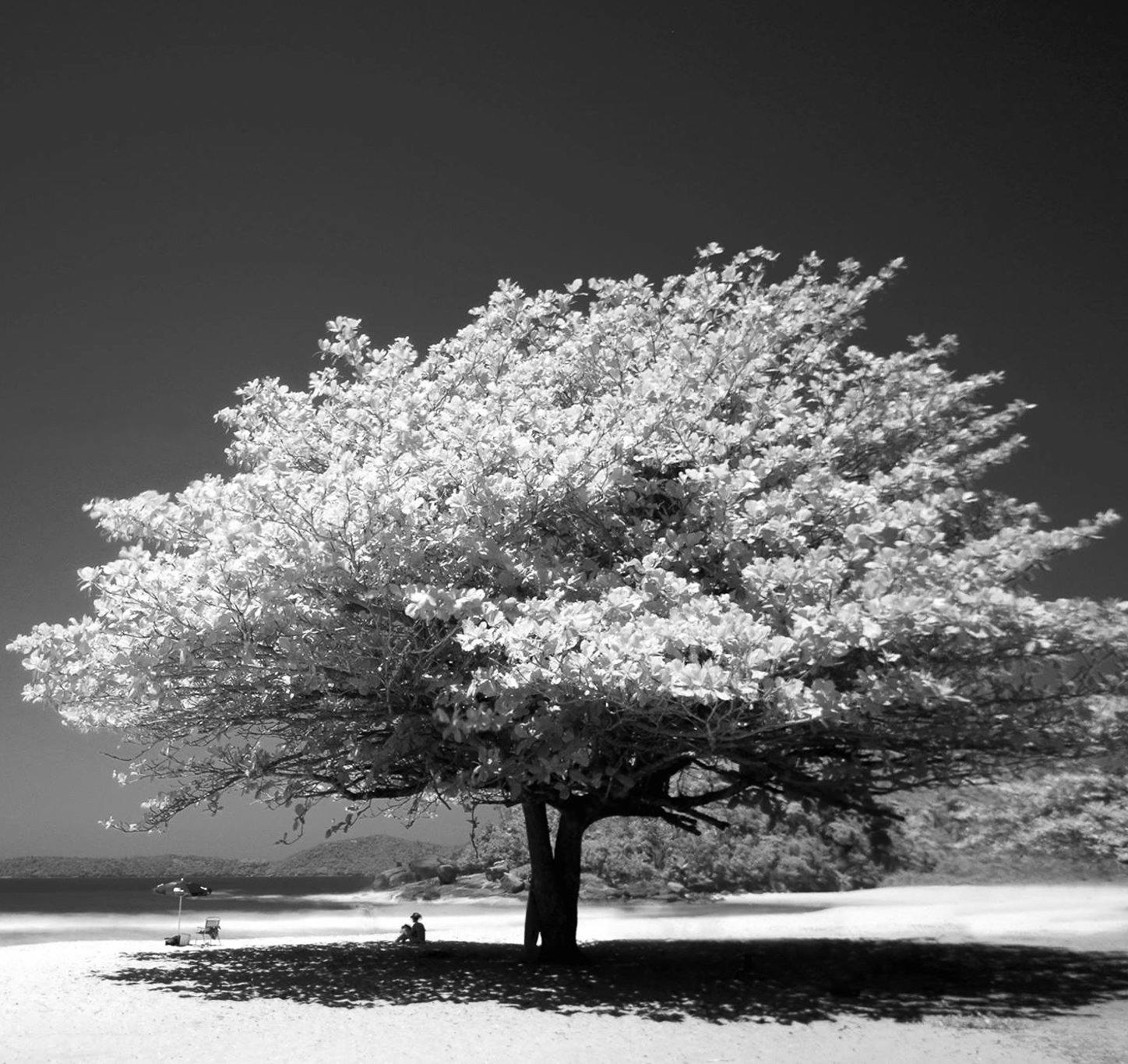
In it, there are uniform areas such as the sky and more complex areas, such as the leaves of the tree. Now look at Figure 2, which shows a $32 imes 32$ pixel patch of sky.

Figure 2. $32 imes 32$ pixel patch of sky
In it we can see that all the pixels are of a very similar color. However, a $32 imes 32$ pixel patch from the area where the tree leaves are located (Figure 3) has a much more complex combination of intensities.

Figure 3. $32 imes 32$ pixel patch of leaves
This becomes even more evident when we look at the pixel values for those areas. In the case of the sky, we can see the following pixels:
>>> import imageio.v3 as iio
>>> I = iio.imread("tree_sky.png")
>>> I[:10, :10, 0]
array([[39, 39, 39, 38, 38, 39, 39, 39, 40, 40],
       [39, 39, 39, 38, 38, 39, 39, 39, 40, 40],
       [39, 39, 39, 38, 38, 39, 39, 39, 40, 40],
       [39, 39, 39, 38, 38, 39, 39, 39, 40, 40],
       [39, 39, 39, 38, 38, 39, 39, 39, 40, 40],
       [39, 39, 39, 38, 38, 39, 39, 39, 40, 40],
       [41, 41, 40, 45, 44, 42, 41, 40, 40, 40],
       [42, 42, 42, 44, 43, 42, 41, 40, 40, 40],
       [43, 43, 42, 44, 43, 42, 40, 40, 39, 40],
       [42, 42, 41, 43, 42, 41, 40, 39, 39, 40]],
       dtype=uint8)
As can be seen, there are a large number of identical pixels. Altering them will produce areas with very similar values with small differences (usually $\pm 1$), which will look suspicious.
On the other hand, the patch corresponding to the leaves does not have an apparent pattern, so it is much more difficult to detect a modification:
>>> import imageio.v3 as iio
>>> I = iio.imread("tree_leaves.png")
>>> I[:10, :10, 0]
array([[131, 145, 134, 145, 146, 135, 128, 119,  90, 119],
       [234, 209,  98, 151, 155, 128,  95, 117, 109, 108],
       [225, 172, 115, 123, 132, 118, 108, 104, 108, 106],
       [179, 147, 139, 132, 112, 112,  97,  95, 109, 112],
       [144, 131, 151, 132, 114, 116,  98,  92, 106, 110],
       [135, 131, 138, 113, 127, 118, 110, 102, 101, 100],
       [120, 124, 119,  92, 107,  99, 110, 110,  98,  95],
       [107, 112, 116, 102,  86,  85, 101, 107,  98,  99],
       [134, 119, 121, 151, 132, 116, 107,  97,  96, 100],
       [180, 140, 125, 198, 207, 164, 123,  92,  92,  96]],
       dtype=uint8)
For this reason, selecting those pixels that are most appropriate for hiding information and avoiding those that are not is one of the techniques that allows a more significant improvement in the undetectability of steganographic methods.
The development of STC (Syndrome Trellis Codes) [Filler:2011:stc], presented in the section Embedding techniques: How to avoid detectable areas, marked the beginning of a new way of doing steganography. STCs make it possible to divide the creation of a steganographic method into two phases: the first, aimed at computing the embedding cost for each pixel, and the second, focused on embedding the message while minimizing the total cost.
In the first phase, the goal is to design a criterion that evaluates how easily a modification in a given pixel could be detected, assigning it a proportional cost. The second phase, in turn, embeds the message so that the sum of the costs of the modified pixels is as small as possible.
Since STCs solve the second phase, creating a new steganographic method based on this methodology is reduced exclusively to designing an appropriate function to compute the embedding cost for each pixel.
Cost computation
Most methods for computing costs in steganography are experimental in nature and lack a solid mathematical basis that precisely indicates which pixels can be modified with a lower risk of detection. Due to this limitation, the most common approach is to try different techniques and validate them through steganalysis, comparing them with other methods. If steganalysis performs worse at detecting our new cost function compared to existing ones, we may consider it more effective.
However, this process is delicate, since experimental results depend largely on the image set used. If we do not have a sufficiently large and diverse database, the results may not be representative, which would lead to the development of cost functions that only work well within a specific image set.
This is a complex problem that is beyond the scope of this book. Nevertheless, we will explore how to build a cost function progressively using filters, an approach widely adopted in the field.
A filter is a mathematical function applied to an image to highlight or attenuate certain characteristics of its pixels. In the context of cost computation in steganography, filters are used to analyze the local structure of the image and determine which regions are more suitable for information embedding without the modifications becoming easily detectable.
Filters can be designed to capture different aspects of the image, such as the presence of edges, textures, or intensity variations. For example, a filter based on intensity differences can help identify homogeneous regions, where a modification might be more noticeable, and distinguish them from areas with high variability, where alterations are less evident.
There are various filters used in image processing to detect specific structures and patterns. Among them, edge detection filters, such as Sobel, make it possible to identify sharp transitions in the image, highlighting structures aligned with specific axes. On the other hand, texture enhancement filters, such as the Laplacian or those based on the analysis of spatial frequencies, highlight local variations in texture, making it easier to identify patterns in the image.
From a mathematical perspective, a filter is usually represented as a convolution operation between the image and a mask (or kernel). The mask defines the transformation applied to each pixel based on its neighbors. For example, in Python this could be done as follows (for a Sobel filter):
import numpy as np
import imageio.v3 as iio
from scipy.signal import convolve2d

def apply_filter(image, kernel):
    return convolve2d(image, kernel, mode='same',
                      boundary='fill', fillvalue=0)

image = iio.imread("tree.png", mode="L")

sobel_x = np.array([[-1, 0, 1],
                    [-2, 0, 2],
                    [-1, 0, 1]])

edges_x = apply_filter(image, sobel_x)
edges_x = np.clip(edges_x, 0, 255).astype(np.uint8)
iio.imwrite("tree_sobel_x.png", edges_x)
However, many image processing libraries already include these filters implemented, so the most common practice is to use them directly instead of programming them from scratch.
Based on what was studied in the previous section, it is clear that we must avoid homogeneous regions, such as the sky, and focus on more complex regions, such as the leaves. Figure 4 shows the result of applying the Sobel filter we implemented in Python to the image in Figure 1.
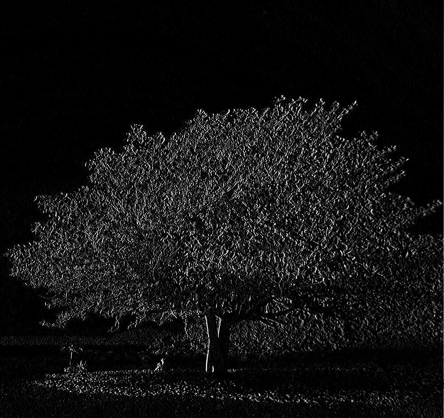
It is a simple filter that is giving us good results, since it clearly differentiates between complex areas (the tree) and simple, flat areas (mainly the sky). However, we have black pixels (values close to zero) in the simple areas, and light pixels (values close to 255) in the complex areas. Since we want a function that tells us the cost of modifying a pixel, we need flat areas to have high costs and complex areas to have low costs, exactly the opposite. Therefore, it is convenient to invert their values. It would be enough to compute 1/edges_x, but since we want to turn it into an image to see how the costs are applied, we will have to normalize it between 0 and 255 to obtain a valid byte value.
import numpy as np
import imageio.v3 as iio
from scipy.signal import convolve2d

def apply_filter(image, kernel):
    return convolve2d(image, kernel, mode='same',
                      boundary='fill', fillvalue=0)

image = iio.imread("tree.png", mode="L")

sobel_x = np.array([[-1, 0, 1],
                    [-2, 0, 2],
                    [-1, 0, 1]])

edges_x = apply_filter(image, sobel_x)
edges_x = np.clip(edges_x, 0, 255).astype(np.uint8)

cost = 1 / edges_x
max_finite = np.max(cost[np.isfinite(cost)])
cost = np.nan_to_num(cost, nan=0, posinf=max_finite, neginf=0)

cost_min, cost_max = cost.min(), cost.max()
cost = np.nan_to_num(cost, nan=0, posinf=cost.max(), neginf=0)

cost_norm = 255 * (cost - cost_min) / (cost_max - cost_min)
cost_norm = cost_norm.astype(np.uint8)

iio.imwrite("tree_sobel_cost.png", cost_norm)
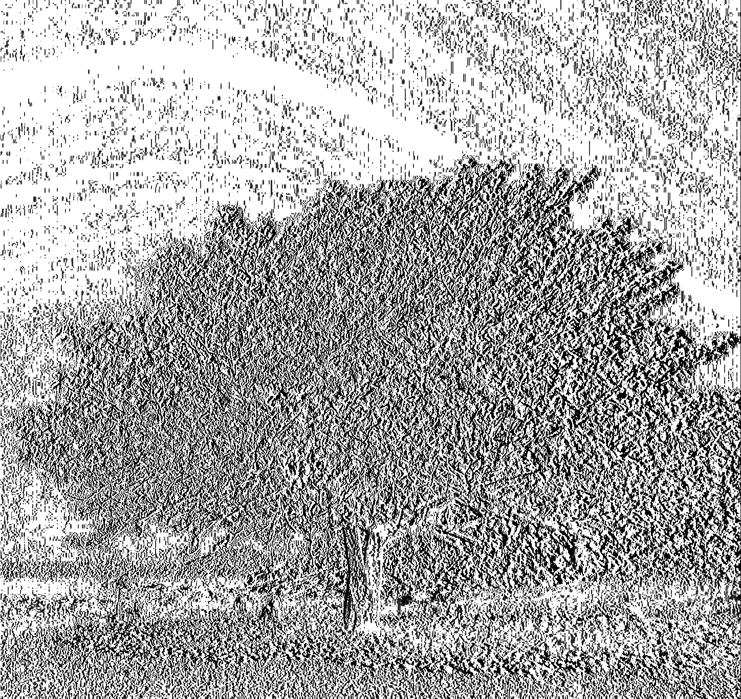
In this way, we obtain a cost function like the one shown in Figure 5. In it, we observe that certain areas of the sky present a maximum cost (255), while regions with greater complexity have lower cost values (close to 0). This confirms that the cost function fulfills its purpose: favoring the embedding of information in the most complex areas of the image.
Although this cost function is useful from a didactic point of view, those used in real applications are usually more complex. They combine multiple filters with various additional strategies. A prominent example is the HILL cost function [Li:2014:hill], which integrates several filters into its formulation.
The reader is encouraged to consult the original article, as it provides a detailed view of the experimental process used to select the optimal combination of filters. Although we will not go into the theoretical details of how HILL works, we will present an implementation in Python.
As in the previous case, we will normalize the values to the range 0 to 255 in order to graphically represent the result.
import numpy as np
import imageio.v3 as iio
from scipy.signal import convolve2d

def HILL(I):
    HF1 = np.array([
        [-1,  2, -1],
        [ 2, -4,  2],
        [-1,  2, -1]
    ])
    H2 = np.ones((3, 3)).astype(np.float32) / 3**2
    HW = np.ones((15, 15)).astype(np.float32) / 15**2

    R1 = convolve2d(I, HF1, mode='same', boundary='symm')
    W1 = convolve2d(np.abs(R1), H2, mode='same', boundary='symm')
    rho = 1.0 / (W1 + 1e-10)
    cost = convolve2d(rho, HW, mode='same', boundary='symm')
    return cost

image = iio.imread("tree.png", mode="L")

cost = HILL(image)
cost = np.nan_to_num(cost, nan=0, posinf=image.max(), neginf=0)

cost_min, cost_max = cost.min(), cost.max()
cost = np.nan_to_num(cost, nan=0, posinf=cost.max(), neginf=0)

cost_norm = 255 * (cost - cost_min) / (cost_max - cost_min)
cost_norm = cost_norm.astype(np.uint8)

iio.imwrite("tree_hill_cost.png", cost_norm)
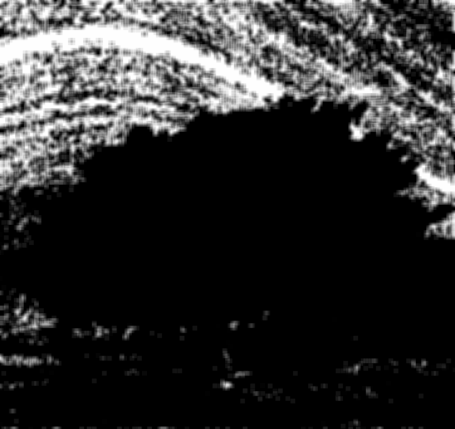
Figure 6 shows the result of applying the HILL cost function. As can be seen, this method clearly identifies the area of the tree as a suitable region for hiding information, while in the sky it detects multiple areas with high sensitivity to modifications, indicating that they are not recommended to be altered.
Syndrome Trellis Codes
In the section Embedding techniques: How to avoid detectable areas we have seen how Syndrome Trellis Codes work and how to use them through the pySTC library. Therefore, applying them to images is quite straightforward. We just need to compute the costs and call the library directly to hide the message.
Below is a Python example using the HILL cost function [Li:2014:hill] that we have seen in the previous section.
In the example we compute the cost with HILL and hide the message Hello World in the image.
import numpy as np
import imageio.v3 as iio
from scipy.signal import convolve2d
import pystc

def HILL(I):
    HF1 = np.array([
        [-1,  2, -1],
        [ 2, -4,  2],
        [-1,  2, -1]
    ])
    H2 = np.ones((3, 3)).astype(np.float32) / 3**2
    HW = np.ones((15, 15)).astype(np.float32) / 15**2

    R1 = convolve2d(I, HF1, mode='same', boundary='symm')
    W1 = convolve2d(np.abs(R1), H2, mode='same', boundary='symm')
    rho = 1.0 / (W1 + 1e-10)
    cost = convolve2d(rho, HW, mode='same', boundary='symm')
    return cost

image = iio.imread("tree.png", mode="L")

costs = HILL(image)

seed = 32  # secret seed
message = "Hello World".encode()
stego = pystc.hide(message, image, costs, costs, seed, mx=255, mn=0)

iio.imwrite("tree_stego.png", stego)
Below we see how to extract the message.
import pystc
import imageio.v3 as iio

stego = iio.imread("tree_stego.png", mode="L")

seed = 32  # secret seed
message_extracted = pystc.unhide(stego, seed).decode()
>>> message_extracted
'Hello World'
It should be noted that the HILL function we have developed operates on a single channel. This is not a problem in our example, since we are working with a grayscale image that contains only one channel. However, to process color images, we could apply HILL independently to each of the channels. Another alternative would be to design a specific function for cost computation in color images that operates directly on all three channels simultaneously.
There are currently no comments on this article.
Add a Comment