Contents
- Compression and Decompression in JPEG
- Access to DCT Coefficients
- Embedding in DCT Coefficients
- Wet Paper Codes
- Adaptive Embedding
- Platform Compression
Compression and Decompression in JPEG
The JPEG format (Joint Photographic Experts Group) is a widely used standard for compressing digital images. It was developed in 1992 by the committee of the same name with the goal of reducing image file size while maintaining acceptable visual quality. Unlike other formats such as PNG or BMP, JPEG uses lossy compression, meaning portions of visual information that are less perceptible to the human eye are discarded to achieve higher compression ratios. This approach significantly reduces file size, making JPEG particularly useful for storage, web transmission, and multimedia applications.
A key feature of JPEG is the ability to control the compression level, allowing a trade‑off between quality and file size. It supports multiple color spaces, such as RGB and YCbCr, and employs techniques like chroma subsampling to optimize compression. However, heavy compression can introduce visual artifacts, including blocking effects or loss of fine texture details.
Thanks to its efficiency and compatibility, JPEG has become the predominant standard for image storage and distribution. It is widely used in digital cameras, mobile phones, and online platforms, where reducing file size is critical to optimize storage and transfer speed. The JPEG compression algorithm has also influenced other image and video coding standards, such as MPEG.
The first step in JPEG compression is to transform the image from the RGB color space to YCbCr. This conversion is used because RGB, while suitable for display, is not optimal for compression. YCbCr separates luminance from chrominance information, enabling compression strategies that reduce file size without significantly affecting perceived visual quality.
In YCbCr space, the Y channel represents luminance (brightness), while Cb and Cr hold chrominance information—the differences of blue and red relative to luminance. The RGB‑to‑YCbCr conversion is a linear combination of the original color channels. The standard conversion equations are:
\(Y = 0.299 R + 0.587 G + 0.114 B\) \(Cb = 128 -0.1687 R - 0.3313 G + 0.5 B\) \(Cr = 128 + 0.5 R - 0.4187 G - 0.0813 B\)
The Y (luminance) channel is the most important for perceived detail because the human eye is more sensitive to brightness variations than color changes. This is leveraged by subsampling in the chrominance channels without an easily perceptible loss of information.
Once the image is converted to YCbCr, the next step is chroma subsampling. This reduces information in the Cb and Cr channels without significantly affecting perceived quality. Because humans are far more sensitive to luminance than chrominance, lowering the resolution of the color components has minimal visual impact.
Chroma subsampling groups adjacent pixels to share color information. Depending on how much Cb/Cr information is retained relative to Y, different subsampling schemes are used. In 4:4:4 there is no reduction—each pixel keeps full color. In 4:2:2, chroma resolution is halved horizontally, so every two pixels share the same color. In 4:2:0, chroma is reduced both horizontally and vertically, so each 2×2 pixel block shares a single Cb/Cr value. The latter is most common in JPEG due to its efficiency with minimal quality loss.
Mathematically, chroma subsampling can be viewed as averaging or discarding values in the chrominance matrices depending on the scheme. With 4:2:0, the Cb and Cr arrays are halved in both dimensions, storing only a quarter of the original color information. During decompression, interpolation reconstructs a visually coherent representation of color.
El submuestreo de crominancia es un paso esencial en la compresión JPEG, ya que permite reducir significativamente la cantidad de datos sin afectar de manera notable la calidad percibida de la imagen. Combinado con la transformada discreta del coseno y la cuantización, este proceso contribuye a obtener archivos de imagen altamente comprimidos con una degradación mínima en su apariencia visual.
After chroma subsampling, JPEG splits the image into 8×8‑pixel blocks. This is fundamental because it enables efficient application of the Discrete Cosine Transform (DCT) to each block, facilitating compression.
The 8×8 block size is a compromise between computational efficiency and compression quality. Each block is processed independently, meaning pixels inside a block influence only that block’s compression and not neighboring blocks. This independence can lead to visible discontinuities between blocks at high compression levels—commonly known as blocking artifacts.
Once the image is partitioned, each block is transformed with the DCT, which represents spatial information in terms of frequencies. This step is essential, enabling removal of redundancy and reducing file size with minimal quality loss.
After applying the DCT to each 8×8 block, we obtain a frequency‑domain representation. Low‑frequency coefficients correspond to the most important variations, whereas high‑frequency coefficients capture fine details. Because the human eye is less sensitive to high frequencies, we can reduce the precision of those coefficients without greatly affecting perceived quality. This step is quantization and accounts for the largest data reduction in JPEG.
Quantization divides each DCT coefficient by a predefined value and rounds the result. Quantization tables assign different precision levels based on position within the block. These values are designed to discard as much high‑frequency information as possible, where losses are less perceptible. Mathematically:
\[Q(u, v) = \text{round} \left( \frac{D(u, v)}{T(u, v)} \right)\]donde $Q(u, v)$ es el coeficiente cuantizado, $D(u, v)$ es el coeficiente DCT original y $T(u, v)$ es el valor correspondiente en la matriz de cuantización.
JPEG typically uses two standard quantization tables—one for luminance and another for chrominance. These tables can be tuned to change the compression level, balancing quality and file size. Higher compression corresponds to larger quantization values, leading to more detail loss but much smaller files.
At high compression levels, quantization artifacts such as blocking and loss of fine textures become visible. Despite this, quantization is essential to JPEG, enabling drastic data reduction without excessive degradation of perceived quality.
After quantization, JPEG organizes and encodes the coefficients to further reduce size. While crucial for compression efficiency, this phase is less relevant for steganography, since data hiding typically manipulates the image in earlier stages.
The first step is to linearize coefficients with a zigzag scan. This orders coefficients from low to high frequency, placing the most significant values at the start and the many post‑quantization zeros at the end. This layout benefits subsequent compression because long zero runs can be represented efficiently.
Once reordered, entropy coding is applied so frequent values use fewer bits. Run‑length encoding compacts zero sequences, followed by Huffman coding, which assigns shorter codes to frequent symbols. This significantly reduces storage without affecting reconstruction.
The final JPEG file combines the encoded data with the information needed for decoding: the quantization tables used, generated Huffman tables, and image metadata. The standardized format ensures any JPEG‑capable software can read and reconstruct the image correctly.
Although essential for compression, this stage has limited relevance to steganography. Most hiding techniques focus on DCT‑coefficient manipulation or direct pixel changes, so entropy coding and file assembly have minor impact. For steganography on already compressed JPEGs, embedding is performed earlier to ensure hidden data survives final coding.
Access to DCT Coefficients
To access the DCT coefficients of a JPEG image, you can use the python-jpeg-toolbox library. The following shows how to load an image, extract its DCT coefficients, and modify them.
The following code loads a JPEG file and accesses its DCT coefficients:
import jpeg_toolbox as jt
import numpy as np
jpeg = jt.load("image.jpeg")
dct_Y = np.array(jpeg['coef_arrays'][0])
dct_Cb = np.array(jpeg['coef_arrays'][1])
dct_Cr = np.array(jpeg['coef_arrays'][2])
If we print the contents of the arrays, we can inspect the DCT coefficients:
>>> dct_Y.shape
(512, 512)
>>> dct_Y[:8,:8]
array([[87.,  2.,  2.,  0.,  0.,  0., -1.,  1.],
       [ 4.,  0.,  0., -2.,  1.,  0.,  0.,  0.],
       [-3.,  0., -1.,  0.,  0.,  0.,  0.,  0.],
       [ 1.,  0.,  0.,  0.,  0.,  0.,  0.,  0.],
       [ 0.,  0.,  0.,  0.,  0.,  0.,  0.,  0.],
       [ 0.,  0.,  0.,  0.,  0.,  0.,  0.,  0.],
       [ 0.,  0.,  0.,  0.,  0.,  0.,  0.,  0.],
       [ 0.,  0.,  0.,  0.,  0.,  0.,  0.,  0.]])
The DCT coefficients are organized into three arrays corresponding to the Y, Cb, and Cr channels. To modify them, you change the desired values and then save the image back to JPEG. In the following code, a coefficient in the luminance channel is changed:
dct_Y[1, 1] = 3
jpeg['coef_arrays'][0] = dct_Y
jt.save(jpeg, "image_stego.jpg")
>>> dct_Y[:8,:8]
array([[87.,  2.,  2.,  0.,  0.,  0., -1.,  1.],
       [ 4.,  3.,  0., -2.,  1.,  0.,  0.,  0.],
       [-3.,  0., -1.,  0.,  0.,  0.,  0.,  0.],
       [ 1.,  0.,  0.,  0.,  0.,  0.,  0.,  0.],
       [ 0.,  0.,  0.,  0.,  0.,  0.,  0.,  0.],
       [ 0.,  0.,  0.,  0.,  0.,  0.,  0.,  0.],
       [ 0.,  0.,  0.,  0.,  0.,  0.,  0.,  0.],
       [ 0.,  0.,  0.,  0.,  0.,  0.,  0.,  0.]])
In addition to DCT coefficients, the library exposes the quantization tables, which determine the compression level. They can be obtained as follows:
>>> jpeg['quant_tables']
array([[[ 3,  2,  2,  3,  4,  6,  8, 10],
        [ 2,  2,  2,  3,  4,  9, 10,  9],
        [ 2,  2,  3,  4,  6,  9, 11,  9],
        [ 2,  3,  4,  5,  8, 14, 13, 10],
        [ 3,  4,  6,  9, 11, 17, 16, 12],
        [ 4,  6,  9, 10, 13, 17, 18, 15],
        [ 8, 10, 12, 14, 16, 19, 19, 16],
        [12, 15, 15, 16, 18, 16, 16, 16]],

       [[ 3,  3,  4,  8, 16, 16, 16, 16],
        [ 3,  3,  4, 11, 16, 16, 16, 16],
        [ 4,  4,  9, 16, 16, 16, 16, 16],
        [ 8, 11, 16, 16, 16, 16, 16, 16],
        [16, 16, 16, 16, 16, 16, 16, 16],
        [16, 16, 16, 16, 16, 16, 16, 16],
        [16, 16, 16, 16, 16, 16, 16, 16],
        [16, 16, 16, 16, 16, 16, 16, 16]]], dtype=int32)
This allows you to analyze the compression used in the image and is also required if you want to implement decompression directly in Python.
Embedding in DCT Coefficients
Introduction
Modifying a DCT coefficient in the frequency domain manifests in the spatial domain after the inverse transform. Because DCT coefficients encode the contribution of different spatial frequencies, altering their values produces changes in the reconstructed image whose magnitude and visibility depend on which coefficient was modified.
Each 8×8 pixel block is decomposed into a combination of spatial frequencies by the DCT. In this representation, coefficients near the top‑left correspond to the lowest frequencies, whereas those toward the bottom‑right are higher frequencies. Low‑frequency coefficients carry most of the block’s visual information; high‑frequency coefficients capture fine details and sharp transitions.
Changing low‑frequency coefficients produces global changes within the corresponding block. In particular, the DC coefficient at (0,0) represents the block’s mean; altering it shifts overall luminance (lighter or darker) without changing internal detail. Modifying high‑frequency coefficients affects fine detail and edges and may introduce visual artifacts (e.g., ripples or noise), making changes more noticeable.
In addition to block‑structure effects, quantization in JPEG influences the outcome of modifications. Quantization reduces the precision of DCT coefficients—particularly at high frequencies—removing details that are less relevant perceptually. As a result, modifications to high‑frequency coefficients may be attenuated or even removed.
When working with DCT coefficients of a JPEG image, it is important to consider the impact of modifying those that are zero. These zeros appear after quantization, which reduces the precision of higher‑frequency values. Many high‑frequency coefficients round to zero, enabling more efficient compression.
Visually, zero‑valued DCT coefficients typically correspond to high‑frequency details such as sharp transitions or fine textures. Modifying them may introduce perceptible variations—unnatural patterns or noise—making changes more detectable to both human observers and steganalysis.
In certain scenarios, modifying zero coefficients might be justified if the embedding scheme accounts for the consequences. In most cases, however, it is preferable to modify nonzero coefficients because the impact on detectability is lower.
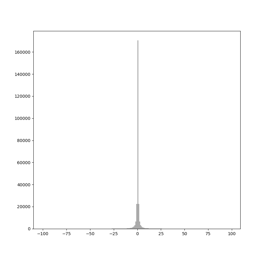
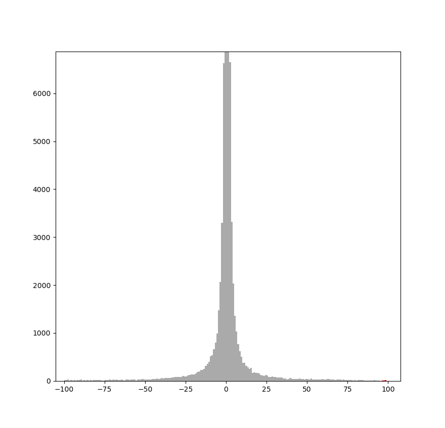
The histogram of DCT coefficients in a JPEG exhibits a characteristic distribution that reflects compression in the transform domain. Generally it is symmetric about zero, since DCT coefficients represent intensity variations that are equally likely to be positive or negative.
This symmetry follows from the DCT’s mathematical structure and the natural frequency distribution of images. Large‑magnitude coefficients are less frequent, while values near zero are far more common because most image energy is concentrated in low frequencies. Quantization accentuates this by reducing high‑frequency precision and rounding many values to zero, reinforcing symmetry.
When DCT coefficients are modified, histogram symmetry can be disturbed depending on the specific changes. For example, a steganographic method that systematically increments or decrements certain coefficients without accounting for the original distribution can bias the histogram so one side of the spectrum predominates over its negative counterpart. Such anomalies are detectable by statistical steganalysis of DCT coefficients.
Figure 1 illustrates the symmetry of the DCT histogram for a sample JPEG. In the full histogram (Fig. 1a), the bar for value 0 is extremely tall. In the zoomed view (Fig. 1b), symmetry is clearer: the bar for coefficients equal to +1 has height similar to −1, +2 similar to −2, and so on.
|
|
La alteración de la simetría del histograma es especialmente relevante en los métodos de esteganografía basados en modificaciones directas de los coeficientes. Si las modificaciones no se distribuyen de manera equilibrada entre los coeficientes positivos y negativos, la estructura estadística de la imagen comprimida se desvía de la que se esperaría en una imagen natural comprimida con JPEG, lo que facilita su detección. Por esta razón, muchas técnicas avanzadas de esteganografía en imágenes JPEG buscan preservar la simetría del histograma o aplicar modificaciones que minimicen su impacto en la distribución de los coeficientes.
En consecuencia, al diseñar métodos de modificación de coeficientes DCT, es fundamental considerar el impacto que estas alteraciones tendrán en la distribución estadística de los coeficientes. Mantener la simetría del histograma o diseñar modificaciones que respeten la estructura natural de los coeficientes DCT puede ser clave para reducir la detectabilidad de la información oculta.
LSB Techniques
The earliest steganographic techniques for JPEG used LSB replacement or matching variants like those discussed in Embedding Techniques: Embedding Bits in the LSB. However, this produced problems similar to embedding data in silent audio regions, as described in Embedding Techniques: How to Avoid Detectable Regions. Modifying zero DCT coefficients by ±1 leads to easily detectable patterns, compromising security.
Furthermore, altering zero‑valued DCT coefficients can cause perceptible changes in the reconstructed image, adding complexity to transform‑domain hiding. To address this effectively, adaptive steganography approaches are essential—optimizing which coefficients to modify to minimize detectability while preserving visual quality.
It is worth noting that early JPEG steganography did not yet employ adaptive methods. As a result, the first techniques relied on ad‑hoc solutions to work around zero‑coefficient issues. We explore some of these strategies next.
Avoiding changes to zero DCT coefficients may sound simple, but it is challenging to do so without introducing statistical anomalies. If we ignore all zero coefficients for embedding, the receiver must do the same during extraction or the message cannot be recovered. This imposes an additional constraint: embedding must not create new zeros; otherwise, those positions will be discarded and information lost.
This issue, known as shrinkage, is easy to illustrate. With LSB matching, embedding into a coefficient with value +1 by applying −1, or into −1 by applying +1, yields 0. Since the receiver ignores zeros, bits embedded at these positions are lost. The well‑known F5 algorithm [westfeld:2001:f5] addresses this by continuing the process and re‑embedding the same bit into the next available coefficient whenever a zero is produced. Although additional zeros are ignored during extraction, the bit can still be found later. The drawback is reduced capacity because some bits must be inserted multiple times.
Another approach avoids creating zeros. Instead of conventional LSB matching, modify coefficients randomly by +1 or −1, except when $|x_i| = 1$. If $x_i = 1$, always apply +1; if $x_i = -1$, always apply −1. This prevents new zeros and ensures correct extraction.
\[x_i' = \begin{cases} x_i + 1, & \text{si } x_i = 1 \\ x_i - 1, & \text{si } x_i = -1 \\ x_i + s, & \text{si } \|x_i\| > 1, \quad \text{donde } s \in \{-1, +1\} \text{ con probabilidad } 0.5 \end{cases}\]However, this alters the DCT‑coefficient histogram: the bars for ±1 decrease relative to neighbors, while the ±2 bars increase, creating a statistical distortion detectable by steganalysis.
Other options exist to embed without creating new zeros, but they typically distort the DCT histogram enough to be detected by simple statistical attacks such as the chi‑square test [westfeld:2000].
Matrix Embedding
As discussed above, preserving the DCT‑histogram distribution without significant anomalies tends to produce new zeros, which complicates extraction because any coefficient turned into zero is lost. To avoid this, F5 [westfeld:2001:f5] re‑embeds the affected bits in later coefficients, at the expense of capacity.
An alternative to mitigate this capacity loss is matrix embedding, which increases embedding efficiency—hiding more information with the same number of coefficient changes.
The following is an example of an F5‑style implementation using matrix embedding with $p=3$, and performing additional embedding whenever a new zero is created.
The matrix embedding part has been discussed previously; here we focus on the embed function, which is somewhat involved.
First, the text message is converted into a bit sequence to be embedded bit by bit. Then we traverse the luminance ($Y$) array.
An important detail is that the DC coefficient (top‑left of each 8×8 block) is ignored. Many steganographic methods do this because DC affects the entire block and can cause noticeable differences relative to neighbors, increasing detectability.
Zero‑valued coefficients are also ignored, as discussed earlier.
Coefficients are read until forming a group of $2^p - 1$, stored in group, which is the size required by the embedding algorithm. For each group of three, we determine which one must be changed to embed the desired bit by decrementing its absolute value by one. This tends to preserve the histogram shape, though it may occasionally create new zeros.
Finally, if a modification creates a new zero, the last element of the group is removed and we continue. Otherwise, the embedding is considered valid and the process proceeds.
import jpeg_toolbox as jt
import numpy as np
import random

P = 3
BLOCK_LEN = 2**P-1
M = np.array([
    [0, 0, 0, 1, 1, 1, 1],
    [0, 1, 1, 0, 0, 1, 1],
    [1, 0, 1, 0, 1, 0, 1]
])

def ME_embed(M, c, m):
    s = c.copy()
    col_to_find = (np.dot(M, c) - m) % 2
    for position, v in enumerate(M.T):
        if np.array_equal(v, col_to_find):
            s[position] = (s[position] + 1) % 2
            break
    return np.array(s)

def embed(img, message):
    dct_Y = img["coef_arrays"][0]

    message_bits = [
        int(bit) for byte in message.encode() for bit in format(byte, '08b')
    ]
    padding = (-len(message_bits)) % P
    message_bits += [0] * padding

    k = 0
    group = []
    for i in range(dct_Y.shape[0]):
        for j in range(dct_Y.shape[1]):
            if k+2 >= len(message_bits):
                break

            # Ignore DC
            if i % 8 == 0 and j % 8 == 0:
                continue

            # ignore zeros
            if dct_Y[i, j] == 0:
                continue

            group.append((i, j))
            if len(group) == BLOCK_LEN:
                m = message_bits[k:k+3]
                cover = np.array([int(dct_Y[a, b]) % 2 for a, b in group])

                stego = ME_embed(M, cover, m)
                idx = np.where(cover - stego != 0)[0]

                # No modifications needed
                if len(idx) == 0:
                    k += P
                    group = []
                    continue

                _i, _j = group[idx[0]]

                # Modify coef
                if dct_Y[_i, _j] < 0:
                    dct_Y[_i, _j] += 1
                else:
                    dct_Y[_i, _j] -= 1

                # Shrinkage
                if dct_Y[_i, _j] != 0:
                    k += P
                    group = []
                else:
                    del group[idx[0]]

    img["coef_arrays"][0] = dct_Y
    return img

img = jt.load("image.jpeg")
message = "Hidden text"
stego_img = embed(img, message)
jt.save(stego_img, "image_stego.jpeg")
Below is the Python code for extracting the hidden message. The procedure is simpler than embedding. We traverse the luminance $Y$ array in the same order used during insertion, discarding DC and zero coefficients. Valid coefficients are grouped into blocks of $2^p - 1$, with each group yielding $p$ bits. The resulting bitstream is finally converted back into the original text message.
As in previous sections, we have not implemented a mechanism to determine when the message ends; in the example we extract the 88 bits we know are present. In practice, one should include a header with the message length or embed an explicit end‑of‑message marker.
import jpeg_toolbox as jt
import numpy as np

class EndLoop(Exception):
    pass

P = 3
BLOCK_LEN = 2**P-1
M = np.array([
    [0, 0, 0, 1, 1, 1, 1],
    [0, 1, 1, 0, 0, 1, 1],
    [1, 0, 1, 0, 1, 0, 1]
])

def ME_extract(M, s):
    return np.dot(M, s) % 2

def extract(img, msglen):
    dct_Y = img["coef_arrays"][0]

    l = msglen + (-msglen) % P
    num_blocks = (l // 3)

    message = []
    p = 3
    group_size = 2**p - 1
    group = []
    try:
        for i in range(dct_Y.shape[0]):
            for j in range(dct_Y.shape[1]):

                # Ignore DC
                if i % 8 == 0 and j % 8 == 0:
                    continue
                # ignore zeros
                if dct_Y[i, j] == 0:
                    continue

                group.append((i, j))
                if len(group) == group_size:
                    stego = np.array([int(dct_Y[a, b]) % 2 for a, b in group])
                    m = ME_extract(M, stego)
                    message += m.tolist()
                    group = []
                    if len(message) >= msglen:
                        raise EndLoop

    except EndLoop:
        pass

    message_bits = ''.join(map(str, message))
    message = ''.join(
        chr(int(message_bits[i:i+8], 2))
        for i in range(0, len(message_bits), 8)
    )

    return message

img = jt.load("image_stego.jpeg")
extracted_message = extract(img, 88)
print(extracted_message)
Wet Paper Codes
In the previous section we analyzed the problem of newly created zeros in JPEG steganography and the F5 solution [westfeld:2001:f5]. While effective, it is not optimal because it requires re‑embedding certain bits, reducing capacity.
A more efficient alternative is to use adaptive embedding techniques that explicitly avoid zero coefficients without re‑insertion. We have explored such techniques earlier. A particularly effective option is Syndrome Trellis Codes (STC), available through the pySTC library. In this case, you define a cost function that heavily penalizes zeros and assigns low cost to the rest. This is straightforward and covered previously.
We define the cost function $C(i,j)$ for a DCT coefficient $x_{i,j}$ as:
\[C(i,j) = \begin{cases} \infty & \text{si } x_{i,j} = 0 \\ 0 & \text{en otro caso} \end{cases}\]Esta función penaliza fuertemente la modificación de coeficientes cuyo valor sea cero, asignándoles un coste infinito. En cambio, permite modificar libremente el resto de coeficientes, asignándoles un coste nulo, independientemente de su valor.
Podemos escribir la función de cálculo de costes de la siguiente manera, en la que asignamos un coste alto, en lugar de infinito:
import numpy as np

def cost(coeffs, high_cost=1e10):
    cost = np.zeros_like(coeffs, dtype=float)
    cost[coeffs == 0] = high_cost
    return cost
This embedding approach eliminates the shrinkage problem discussed earlier and is therefore known as non‑shrinkage F5 or nsF5 [Fridrich:2007:nsF5].
While effective against the F5 problem, this does not fully align with adaptive JPEG steganography principles. The objective, discussed elsewhere, is to select regions where embedding is hardest to detect. We address this in more depth next.
Adaptive Embedding
In previous chapters we studied cost functions that adapt to image regions that are difficult to model statistically, and are therefore better suited for hiding information stealthily. The same ideas apply here because analysis of the decompressed image remains relevant.
In other words, we can modify DCT coefficients, decompress the image, and study how the resulting pixels are affected to determine whether we changed areas we would prefer to avoid. This adds complexity: we must compute cost in the DCT domain and evaluate the impact after decompression.
The main drawback is computational cost. If each 8×8 block requires decompression to evaluate pixel‑domain effects, the number of operations grows significantly—especially if implemented in pure Python.
For this reason, the limiting factors are often practical rather than theoretical. More accurate cost functions may exist in theory, but real‑world application can be constrained by performance.
It is therefore important not only to design good cost functions but also to pair them with tools that improve computational efficiency. The Numba library is recommended for JIT‑compiling critical sections and significantly accelerating execution.
An especially effective algorithm for computing a JPEG cost function is J‑UNIWARD [Holub:2014:uniward]. While beyond this book’s scope, we sketch the main ideas. Reference implementations are available at:
https://github.com/daniellerch/stegolab/tree/master/J-UNIWARD
For learning, start with j-uniward.py (grayscale). Once understood, continue with j-uniward-color.py for color images. As noted earlier, the process can be computationally expensive; j-uniwardfast-color.py demonstrates using Numba to accelerate it.
The main idea behind J‑UNIWARD is to evaluate the pixel‑domain impact of changing each DCT coefficient. It computes the cost of such modifications in the decompressed image as follows:
import scipy.fftpack
import numpy as np

def idct2(a):
    return scipy.fftpack.idct(scipy.fftpack.idct(a, axis=0, norm='ortho'),
                              axis=1, norm='ortho')

# ...
spatial_impact = {}
for i in range(8):
    for j in range(8):
        test_coeffs = np.zeros((8, 8))
        test_coeffs[i, j] = 1
        spatial_impact[i, j] = idct2(test_coeffs) * jpg["quant_tables"][0][i, j]
# ...
This allows a cost function to be applied in the decompressed image. J‑UNIWARD uses a different function than HILL [Li:2014:hill]—based on wavelet filters—but the principle is the same:
import scipy.signal

# ...
wavelet_impact = {}
for f_index in range(len(F)):
    for i in range(8):
        for j in range(8):
            wavelet_impact[f_index, i, j] = scipy.signal.correlate2d(
                spatial_impact[i, j], F[f_index],
                mode='full', boundary='fill',
                fillvalue=0.0
            )
# ...
In summary, adaptive JPEG steganography assigns a cost to each coefficient that reflects the impact of modifying it on the decompressed image. With this cost map, STC can be applied to the coefficients.
Platform Compression
Many social networks, messaging apps, and forums automatically apply lossy compression—mainly JPEG—to uploaded images. This reduces file sizes, improving storage efficiency and transfer speed. From a steganography standpoint, however, it is a direct threat: any technique that relies on exact pixel values or DCT coefficients may be destroyed by platform recompression.
If a message is embedded in an uncompressed image (e.g., PNG or BMP) and the platform converts it to JPEG, LSB‑based hidden data is lost. The transform to the DCT domain followed by quantization alters the data completely. Even if the image is already JPEG, recompression can still destroy hidden content whenever the platform’s quality setting differs from the sender’s; re‑quantization changes the DCT coefficients, eliminating or distorting embedded bits.
To mitigate this, a simple yet effective tactic is to pre‑compress with the same quality the platform will apply. If the platform’s JPEG quality is known, compress the image accordingly and then apply a JPEG‑domain steganographic method such as nsF5 [Fridrich:2007:nsF5] or J‑UNIWARD [Holub:2014:uniward]. The platform’s compression will then leave the original coefficients unchanged and the hidden message intact. For example, if a platform uses ≈85% JPEG quality, first convert your image to JPEG at ≈85% and only then embed using nsF5 or J‑UNIWARD.
There are currently no comments on this article.
Add a Comment